Finite Pattern Entropy: Understanding Information in Limited Sequences

PDF

Zsolt Pocze

Abstract

A unified combinatorial definition of the information content and entropy of different types of patterns, compatible with the traditional concepts of information and entropy, going beyond the limitations of Shannon information interpretable for ergodic Markov processes. We compare the information content of various finite patterns and derive general properties of information quantity from these comparisons. Using these properties, we define normalized information estimation methods based on compression algorithms and Kolmogorov complexity. From a combinatorial point of view, we redefine the concept of entropy in a way that is asymptotically compatible with traditional entropy.

1 Introduction

The characteristic feature of a material is its pattern, which we interpret broadly as the arrangement of its elementary components. This also includes the relationships between individual parts. In physical reality, every finite-dimensional pattern can be modeled, with some accuracy, as a one-dimensional finite sequence. Therefore, we examine information and entropy in relation to finite sequences (patterns). Let

X^{*}

denote the set of finite patterns, where

X

is the value set (or base set) of the patterns. For a given pattern

A \in X^{*}

A = (x_{1}, x_{2}, …, x_{n})

, let

n = | A |

be the length of the pattern,

k = | X |

be the number of elements in the value set, and let

f (x)

x \in X

be the number of occurrences of the element

x

in the pattern.

Information is nothing other than the number of binary decisions [6], required to uniquely determine a pattern, i.e., the number of decisions needed to select the given pattern from among all possible patterns and the empty pattern. The fundamental unit of information is the binary decision, measured in bits. In practice, the number of decisions can only take integer values, but if we use a continuous function, we do not always obtain integer values; this yields the theoretical number of decisions. For the sake of mathematical simplicity, we will hereafter always refer to the theoretical number of decisions as the number of decisions. For this reason, and others, determining the amount of information is always an approximate process.

Definition 1. Let the information of a finite pattern

A \in X^{*}

be the minimum number of binary decisions necessary to uniquely specify that pattern. Denote this by

I (A)

, where

I : X^{*} \to R^{+}

is a function, and

\begin{matrix} I (A) = m i n {n | A i s r e p r o d u c i b l e b y d e c i s i o n s e q u e n c e (d_{1}, d_{2}, …, d_{n})} boxempty & (1) \end{matrix}

This definition is general since it does not depend on any specific system, purely theoretical since it explicitly incorporates all implicit information, and is philosophically less debatable because the minimum number of decisions represents the most general measure of information content. At the same time, the concepts within the definition are not precisely defined for practical or even theoretical application: we have not fixed what exactly constitutes an elementary decision, what reproducibility means, nor how to decompose the description of generating a pattern into elementary decisions.

Kolmogorov complexity [4] is a special case of the above definition of information, which determines the number of decisions required to describe patterns using a universal Turing machine:

Definition 2. Let

U

be a fixed universal Turing machine. Then, the Kolmogorov complexity

I_{K} (A)

of a finite pattern

A \in X^{*}

is defined as:

\begin{matrix} I_{K} (A) = m i n {∣ B ∣ : U (B) = A} & (2) \end{matrix}

where

∣ B ∣

denotes the length of the binary program (bit sequence), and the minimum is taken over all programs

B

that, when used as input to the universal Turing machine

U

, produce

A

as output.

Unfortunately, Kolmogorov complexity is generally not computable [1]. However, the information content can be determined very precisely and explicitly in certain edge cases. These include numbers, constant patterns, uniformly distributed random patterns, and patterns with well-defined statistical properties, such as those generated by ergodic Markov processes.

When seeking more accurate methods for defining information in both theoretical and practical contexts, it is essential to first examine these edge cases and the aforementioned special instances.

2 Information Content of a Constant Pattern

For a constant and finite pattern

A \in {a}^{*}

, no information is required to determine the individual elements of the pattern since it consists of the repetition of a single element. Only the length of the pattern,

n

, carries information, which requires at most

⌈ l o g_{2} n ⌉

decisions (or bits of information) to determine, as each decision halves the possible options. For simplicity and mathematical tractability, we use the theoretical approximation

l o g_{2} n

Starting from the information content of integers, one can calculate the information content of any pattern composed of identical elements if we interpret information as the process of selecting the given pattern from all possible sub-patterns, including the zero-length pattern.

$1$	$()$
$2$	$a$
$3$	$a a$
…	…
$n + 1$	$a a a … a$

Table 1: In the case of a constant pattern of length

n

, the definition of information can be simplified to selecting from

n + 1

elements, where

()

denotes the empty pattern.

The logarithm of the total number of possible patterns that can be formed from the elements of the pattern gives the information content of the specific pattern. In that case, the information of

A

is:

\begin{matrix} I_{c o n s t} (A) = l o g_{2} (n + 1) & (3) \end{matrix}

Using

n + 1

instead of

n

is more practical because it allows the information content of an empty pattern to be defined, acknowledging that the empty pattern, as a possibility, also carries information. It is easy to see that among finite patterns, constant patterns have the lowest information content, as non-constant patterns require more decisions due to the presence of different elements. These additional decisions increase the information content.

We do not use the formula

l o g_{2} (n)

because then subadditivity is not satisfied for patterns of length one. The condition for subadditivity is

I_{r a n d} (a b) \leq I_{r a n d} (a) + I_{r a n d} (b)

. If we used the formula

l o g_{2} n

, then for the concatenation of patterns of length

n = 1

, subadditivity would not be satisfied:

l o g_{2} (2) ≰ l o g_{2} (1) + l o g_{2} (1)

. In the case of the formula

l o g_{2} (n + 1)

, however, subadditivity is satisfied for all

n \geq 0

$n_{1}$	$n_{2}$	Subadditivity
$0$	$0$	$l o g_{2} 1 \leq l o g_{2} 1 + l o g_{2} 1$
$0$	$1$	$l o g_{2} 2 \leq l o g_{2} 1 + l o g_{2} 2$
$1$	$1$	$l o g_{2} 3 \leq l o g_{2} 2 + l o g_{2} 2$
$1$	$2$	$l o g_{2} 4 \leq l o g_{2} 2 + l o g_{2} 3$
$2$	$2$	$l o g_{2} 5 \leq l o g_{2} 3 + l o g_{2} 3$

Table 2: The fulfillment of subadditivity in the case of uniformly distributed random sequences of different lengths.

3 Information Content of a Uniformly Distributed Random Pattern

A finite pattern

A \in X^{*}

with a uniform distribution can be generated such that each element of the pattern results from an independent decision requiring

l o g_{2} (k)

bits, where

k

is the number of possible symbols. Considering that we can select from

n + 1

patterns of different lengths, the pattern’s information content is:

\begin{matrix} I_{r a n d} (A) = l o g_{2} \sum_{i = 0}^{n} k^{i} & (4) \end{matrix}

k = 1

, i.e., if

A

is a constant pattern, the formula simplifies to the constant pattern formula:

I_{r a n d} (A) = l o g_{2} \sum_{i = 0}^{n} 1^{i} = l o g_{2} (n + 1)

The complexity of

I_{r a n d} (A) = l o g_{2} \sum_{i = 0}^{n} k^{i} = l o g_{2} \frac{k^{n + 1} - 1}{k - 1}

O (n \cdot l o g_{2} (k))

, Thus, for sufficiently large

n

and

k

, the approximation

I_{r a n d} (A) \approx n \cdot l o g_{2} (k)

also holds. We do not use the formula

n \cdot l o g_{2} (k)

because, in the case of unit-length patterns, subadditivity would not hold:

2 \cdot l o g_{2} (2) ≰ 1 \cdot l o g_{2} (1) + 1 \cdot l o g_{2} (1)

and it would not yield accurate values for constant patterns either.

4 Information Content of Patterns Generated by an Ergodic Markov Process

Let

A \in X^{*}

be a pattern that can be generated by an ergodic Markov process, and let

f_{r e l} (x_{i}) = \frac{f (x_{i})}{n}

x_{i} \in X

i = 1, …, k

be the relative frequencies of the values in the pattern. Shannon’s original formula

I_{S h a n n o n} (A) = n \cdot \sum_{i = 1}^{k} f_{r e l} (x_{i}) l o g_{2} \frac{1}{f_{r e l} (x i)}

[6] would not be compatible with the formulas for uniformly distributed patterns and constant patterns, so it needs to be adjusted. Then, by modifying Shannon’s formula, the information of the pattern is:

\begin{matrix} I_{m a r k} (A) = l o g_{2} \sum_{i = 0}^{n} \prod_{x \in X} f_{r e l} (x)^{- i \cdot f_{r e l} (x)} & (5) \end{matrix}

k = 1

, i.e.,

A

is a constant pattern, meaning

f_{r e l} (x) = 1

x \in X

, the formula simplifies to the constant pattern formula:

I_{m a r k} (A) = l o g_{2} \sum_{i = 0}^{n} \prod_{x \in X} 1^{- i} = l o g_{2} (n + 1)

For a pattern generated by a uniformly distributed process, where

f_{r e l} (x_{i}) = \frac{1}{k}

x_{i} \in X

i = 1, …, k

, i.e., all values have identical relative frequencies, the formula simplifies to the information formula for a uniformly distributed pattern:

I_{m a r k} (A) = l o g_{2} \sum_{i = 0}^{n} \prod_{x \in X} (\frac{1}{k})^{- i \cdot \frac{1}{k}} = l o g_{2} \sum_{i = 0}^{n} \prod_{x \in X} k^{i \cdot \frac{1}{k}} = l o g_{2} \sum_{i = 0}^{n} k^{i}

It can be seen that

l i m_{n \to \infty} I_{m a r k} (A) = I_{S h a n n o n}

. Let be

c = \prod_{x \in X} f_{r e l} (x)^{- f_{r e l} (x)}

. If

n \to \infty

, then

I_{m a r k} (A) = l o g_{2} \sum_{i = 0}^{n} c^{i} \approx l o g_{2} (\frac{c^{n + 1} - 1}{c - 1}) \approx n \cdot l o g_{2} c

. It follows that

I_{m a r k} (A) \approx n \cdot l o g_{2} \prod_{x \in X} f_{r e l} (x)^{- f_{r e l} (x)}

, which, based on the properties of logarithms can be written to

I_{m a r k} (A) \approx n \cdot \sum_{x \in X} l o g_{2} (f_{r e l} (x)^{- f_{r e l} (x)})

, which can be further rewritten as

I_{m a r k} (A) \approx n \cdot \sum_{x \in X} f_{r e l} (x) \cdot l o g_{2} (\frac{1}{f_{r e l} (x)}) = I_{S h a n n o n} (A)

Theorem 1. For finite patterns that can be generated by an ergodic Markov process, the value of

I_{m a r k} (A)

is maximized precisely when the relative frequencies of the values are equal, i.e.,

f_{r e l} (x) = \frac{1}{k}, \forall x \in X boxempty

The information-measuring formula can be rewritten using a logarithm in the form

I_{m a r k} (A) = l o g_{2} \sum_{i = 0}^{n} 2^{- i \sum_{x \in X} f_{r e l} (x) l o g_{2} f_{r e l} (x)}

. Because the function

- l o g_{2} x

is convex, we can apply Jensen’s inequality:

\sum_{x \in X} f_{r e l} (x) l o g_{2} f_{r e l} (x) \leq l o g_{2} (\sum_{x \in X} f_{r e l} (x) \cdot 1)

, which simplifies to

\sum_{x \in X} f_{r e l} (x) l o g_{2} f_{r e l} (x) \leq 0

. Equality holds if and only if all

f_{r e l} (x)

values are the same, i.e.,

f_{r e l} (x) = \frac{1}{k}, \forall x \in X

. Therefore, the information content of finite patterns produced by ergodic Markov processes is exactly maximized when every value appears with the same frequency in the pattern, and it follows that uniformly distributed random patterns have the maximum amount of information, with information content

l o g_{2} \sum_{i = 0}^{n} k^{i}

Shannon defined information for ergodic Markov processes [6], but it is important to note that in practice, a significant portion of patterns cannot be generated by an ergodic Markov process, so Shannon’s formula cannot be used to measure information and entropy in those cases. Among all possible finite patterns, only a relatively small subset can be generated by an ergodic Markov process. The reason is that patterns generated by ergodic Markov processes must satisfy certain statistical properties and transition probabilities. Kolmogorov [4] offers a more general solution than Shannon’s method. In contrast to Shannon information, Kolmogorov complexity can be defined for every possible finite pattern.

5 Information Content of General Patterns

5.1 General Properties of Information

From the information of specific patterns, we can infer the general properties of information [3]. The following statement is easy to see:

Theorem 2. Let

A \in X^{*}

be a pattern, let

B \in X^{*}

a constant pattern,

C \in X^{*}

a random pattern, and

| A | = | B | = | C |

. Then the following inequality holds:

\begin{matrix} I_{c o n s t} (B) \leq I (A) \leq I_{K} (A) \leq I_{m a r k} (A) \leq I_{r a n d} (C) boxempty & (6) \end{matrix}

The information content

I_{r a n d}

of a random pattern is the largest, while the information content

I_{c o n s t}

of a constant pattern is the smallest. Since Kolmogorov complexity is based on Turing machines, it cannot always provide a description of a finite pattern as concise as might be achievable using other methods without a Turing machine:

I_{K}

closely approximates the information content but can be larger. The modified Shannon information

I_{m a r k}

, optimized for ergodic Markov sequences, overestimates the information content for non-ergodic and non-Markov processes and yields higher values for less random patterns.

Theorem 3. The general properties of information:

Normalization: $l o g_{2} (n + 1) \leq I (A) \leq l o g_{2} \sum_{i = 0}^{n} k^{i}$ , for any $A \in X^{n}$ and $n \in N^{+}$ .
Subadditivity: $I (A B) \leq I (A) + I (B)$ , for any $A, B \in X^{*}$ .
Reversibility: $| I (A) - I (A^{R}) | \leq c$ , for some $c \in R_{0}^{+}$ , where $A^{R} [i] = A [n - i]$ , $\forall i \in {1, …, n}$ , for $A \in X^{*}$ .
Monotonicity: $I (A) \leq I (B)$ , for any $A, B \in X^{*}$ , if $A$ is a subpattern of $B$ .
Redundancy: $| I (A^{r}) - (I (A) + l o g_{2} (r)) | < c$ , for some $c \in R_{0}^{+}$ , where $A^{r}$ denotes the pattern $A$ repeated $r$ times. $boxempty$

The normalization property follows from the information of the constant pattern

I_{c o n s t} (A) = l o g_{2} (n + 1)

and the uniformly distributed random pattern

I_{r a n d} (A) = l o g_{2} \sum_{i = 0}^{n} k^{i}

, as well as from Statement 1.

Subadditivity can be easily seen in the case of a constant pattern:

l o g_{2} (n + m + 1) \leq l o g_{2} (n + 1) + l o g_{2} (m + 1)

, which, when rearranged, becomes

l o g_{2} (n + m + 1) \leq l o g_{2} (n \cdot m + n + m + 1)

, and this holds in every case. For ergodic Markov processes, let

C = \prod_{x \in X} f_{r e l} (x)^{f (x)}

, then the inequality

l o g_{2} \sum_{i = 0}^{n + m} C^{- i} \leq l o g_{2} \sum_{i = 0}^{n} C^{- i} + l o g_{2} \sum_{i = 0}^{m} C^{- i},

can be rewritten as

\sum_{i = 0}^{n + m} C^{- i} \leq (\sum_{i = 0}^{n} C^{- i}) (\sum_{i = 0}^{m} C^{- i})

. Rewriting the right-hand side gives

\sum_{i = 0}^{n + m} C^{- i} \leq \sum_{i = 0}^{n} \sum_{j = 0}^{m} C^{- (i + j)} = \sum_{i = 0}^{n + m} (\sum_{k, l; k + l = i} C^{- i})

. For every

k

, there is at least one

(k, l)

pair that satisfies the conditions, which means the inner sums include the term

C^{- k}

at least once. Therefore, the inequality holds.

Reversibility means that it makes no difference from which side we start reading the pattern—it does not affect its information content. This is trivial, because the interpreter can easily reverse the pattern. Monotonicity is similarly trivial for both constant patterns and those generated by an ergodic Markov process.

Let

A^{r} = A A … A

be a redundant pattern of length

n r

. Then

I_{c o n s t} (A^{r}) = l o g_{2} (n r + 1) = l o g_{2} (n + 1) + l o g_{2} r + l o g_{2} (\frac{n r + 1}{(n + 1) r})

. The expression

l o g_{2} (\frac{n r + 1}{(n + 1) r})

approaches

0

n

and

r

grow, meaning it is bounded. Hence, there always exists some

c \in R_{0}

, such that

| I (A^{r}) - (I (A) + l o g_{2} (r)) | < c

. In the case of random and ergodic Markov processes—and more generally as well—this relationship can be seen intuitively.

Definition 3. Let

A \in X^{*}

be a finite pattern. Its minimum information is given by the function

I_{m i n} : X^{*} \to R^{+}

I_{m i n} (A) = l o g_{2} (n + 1)

and its maximum information is given by the function

I_{m a x} : X^{*} \to R^{+}

I_{m a x} (A) = l o g_{2} \sum_{i = 0}^{n} k^{i} boxempty

5.2 Calculating Information Based on Kolmogorov Complexity

The general definition of information introduced in Definition 1 is closely related to the Kolmogorov complexity specified in Definition 2 [4], Kolmogorov complexity defines the information content of patterns on a given universal machine as the length of the shortest binary program code that generates these patterns.

Fixing the universal machine in Kolmogorov complexity ensures that the information of different patterns can be compared, because there may be a constant difference between the results of various universal machines. This difference becomes negligible for longer patterns but can be significant for shorter ones. The relationship between information and Kolmogorov complexity can be described by the formula

K (A) = I (A) + c

[2], where

c

is a constant characteristic of the universal machine used to compute

K

. Since we know the minimum information

I_{m i n} (A)

precisely, we can eliminate the constant difference and determine how to measure information based on Kolmogorov complexity:

Definition 4. Let

A \in X^{*}

be a pattern. The information of

A

measured by Kolmogorov complexity is defined as

\begin{matrix} I_{K} (A) = K (A) - K_{m i n} (A) + I_{m i n} (A) & (7) \end{matrix}

where

K_{m i n} (A)

is the Kolmogorov complexity of a constant pattern of length

n

K_{m i n} (A) = K ({a}^{n}) boxempty

5.3 Calculating Information Based on a Compression Algorithm

However, for general patterns, it is theoretically impossible to determine Kolmogorov complexity (i.e., the exact amount of information) precisely—only approximations are possible. Lossless compression algorithms are the best approach for this [5]. When a pattern is compressed using such algorithms, it becomes almost random due to its high information density. If we measure the information content of the compressed pattern by assuming it is random, we obtain an approximation of the original pattern’s information content. A characteristic feature of compression algorithms is that the decompression algorithm and additional data are often included in the compressed code. For smaller patterns, this can represent a relatively large amount of extra information, so the resulting information must be normalized.

Definition 5. A function

C : X^{*} \to X^{*}

is called a compression if:

$C$ is injective, that is, if $A, B \in X^{*}$ and $C (A) = C (B)$ then $A = B$ .
For every $A \in X^{*}$ , $∣ C (A) ∣ \leq ∣ A ∣$ .
There is at least one $A \in X^{*}$ , such that $∣ C (A) ∣ < ∣ A ∣$ . $boxempty$

For simplicity, we define the compression function so that the set of possible values for uncompressed and compressed patterns is the same.

Theorem 4. If

C : X^{*} \to X^{*}

is a compression, then

I (A) \leq C (A)

for any

A \in X^{*}

Definition 6. Let

A \in X^{n}

be an arbitrary pattern, and let

C : X^{*} \to X^{*}

be any compression algorithm. Then the information of

A

measured by the compression algorithm

C

is given by:

I_{C} (A) = \frac{I_{m a x} C (A) - I_{m i n}^{C} (A)}{I_{m a x}^{C} (A) - I_{m i n}^{C} (A)} \cdot I_{m a x} (A) + I_{m i n} (A)

where

I_{m i n}^{C} (A) = min_{A \in X^{n}} I_{m a x} (C (A))

I_{m a x}^{C} (A) = max_{A \in X^{n}} I_{m a x} (C (A)) boxempty

Although determining

I_{m i n}^{C}

and

I_{m a x}^{C}

directly from the definition may appear cumbersome in practice, if we take into account that compressed patterns—due to their high information density—are almost random and can therefore be well-modeled by a Markov process, we may use the following approximation:

I_{m i n}^{C} (A) = I_{m a r k} (C (B))

I_{m a x}^{C} (A) = I_{m a r k} (C (D))

where

B \in X^{n}

is an arbitrary constant pattern, and

D \in X^{n}

is any uniformly distributed random pattern.

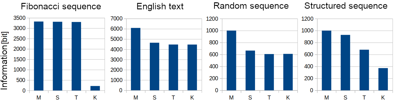Figure 1: In the figure, we can see a comparison of the information values of various 1,000-character-long patterns (APPENDIX I) that differ in their sets of possible symbols. M denotes the maximum amount of information possible for a pattern of the given length and symbol set. S is the pattern’s modified Shannon information. T is the pattern’s information as measured by the GZip compression algorithm. K is the pattern’s approximate Kolmogorov complexity. The “random pattern” is a random binary pattern with a certain degree of redundancy, whereas the “structured pattern” is a 40×25 binary character matrix in which the ‘1’ symbols are arranged in concentric circles.It is apparent that, because of its seeming randomness, even the compression algorithm could not determine the Fibonacci sequence’s information content, whereas its Kolmogorov complexity indicated a low information content. For the English text and the random pattern, both the Shannon-based method and the compression algorithm provided good results. In the case of structured text, however, the compression algorithm clearly gives a closer approximation of the real information content than the Shannon formula, which was originally designed for random patterns. (The algorithms used are described in APPENDIX II–IV.)

Different information measurement methods have varying levels of effectiveness for different structures, so higher accuracy can be achieved by taking the minimum of the results obtained from several measurement methods.

Definition 7. Let

(I_{1}, I_{2}, …, I_{m})

be information measurement methods, and let

A \in X^{n}

be a pattern. The information of

A

, measured using th

I_{m}

methods, is defined as:

\begin{matrix} I_{m} (A) = min_{i = 1, …, m} I_{i} (A) boxempty & (8) \end{matrix}

6 Entropy of Finite Patterns

Unlike information, entropy is an average characteristic of a pattern, meaning the average amount of information required to specify a single element. In most cases, entropy is (incorrectly) identified with Shannon entropy [7], which only approximates the per-element average information content well in the case of ergodic Markov processes. Entropy calculated from Kolmogorov complexity offers a better approximation and is more general, so it is more appropriate to define entropy based on information content, where the method of measuring that information is not predetermined.

A \in X^{*}

is a constant pattern,

X = {a}

, and

()

denotes the empty pattern, entropy can be interpreted from a combinatorial point of view, taking into account the empty pattern as follows:

n	Pattern	Entropy
$0$	$()$	$l o g_{2} (1)$
$1$	$() (a)$	$l o g_{2} (2) / 2$
$2$	$() (a) (a)$	$l o g_{2} (3) / 3$

Table 3: Entropy of the contant patterns.

In general, entropy can be defined in this combinatorical interpretation as follows.

Definition 8. Let

A \in X^{*}

be a finite pattern. The entropy

H_{C} : X^{*} \to R^{+}

of the pattern is the average information content of its elements, namely:

\begin{matrix} H_{C} (A) = \frac{I (A)}{n + 1} & (9) \end{matrix}

where

I

denotes an information measurement method.

boxempty

The factor

n + 1

in the denominator allows the formula to be interpreted for empty patterns. For a constant pattern

A \in X^{*}

where

| X | = 1

, we have

H_{C} (A) = \frac{l o g_{2} (n + 1)}{n + 1}

, This means that as

n

increases, the entropy asymptotically approaches zero.

In the case of ergodic Markov processes, the entropy converges to the Shannon entropy as

n

increases:

l i m_{n \to \infty} H_{C} (A) = H (A)

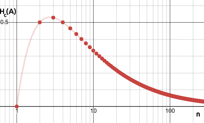
Figure 2: Entropy of a constant pattern as a function of

n

7 Summary

This paper offers a unifying view of information and entropy measures for finite patterns that goes beyond the conventional Shannon framework. By comparing established methods like Shannon’s entropy for ergodic Markov processes with more general approaches such as Kolmogorov complexity, it provides a broader perspective on measuring information content under diverse structural conditions. Fundamental definitions for constant, random, and Markov-generated patterns are introduced, alongside general properties like subadditivity and redundancy. While traditional methods frequently yield imprecise estimates for short patterns, the framework presented here, supported by also practical, compression-based techniques, remains robust even for very short sequences and bridges theoretical concepts with real-world applications. This unified treatment of different notions of entropy clarifies their suitability across various data types, and offers mathematicians, computer scientists, and those interested in advanced data analysis or information theory a wealth of clear examples, formal proofs, and innovative insights into both well-known and less-explored approaches for quantifying information in finite sequences.

References

1Gregory J. Chaitin, “On the Length of Programs for Computing Finite Binary Sequences“, J. ACM 13, 4 (1966), pp. 547–569.

2Gregory J. Chaitin, “A Theory of Program Size Formally Identical to Information Theory“, Journal of the ACM (JACM) 22, 3 (1974), pp. 329–340.

3Thomas M. Cover and Joy A. Thomas, Elements of Information Theory 2nd (Wiley-Interscience, 2006).

4A. N. Kolmogorov, “On tables of random numbers“, Mathematical Reviews (1963).

5Ming Li and Paul Vitányi, An Introduction to Kolmogorov Complexity and Its Applications 2nd (Springer, 1997).

6Claude E. Shannon, “A Mathematical Theory of Communication“, Bell System Technical Journal (1948).

7Claude E. Shannon and Warren Weaver, The Mathematical Theory of Communication (University of Illinois Press, 1949).

APPENDIX I.

The 1,000-character-long patterns used for the comparison shown in Figure 1.

Fibonacci sequence

0 1 2 3 5 8 1 3 2 1 3 4 5 5 8 9 1 4 4 2 3 3 3 7 7 6 1 0 9 8 7 1 5 9 7 2 5 8 4 4 1 8 1 6 7 6 5 1 0 9 4 6 1 7 7 1 1 2 8 6 5 7 4 6 3 6 8 7 5 0 2 5 1 2 1 3 9 3 1 9 6 4 1 8 3 1 7 8 1 1 5 1 4 2 2 9 8 3 2 0 4 0 1 3 4 6 2 6 9 2 1 7 8 3 0 9 3 5 2 4 5 7 8 5 7 0 2 8 8 7 9 2 2 7 4 6 5 1 4 9 3 0 3 5 2 2 4 1 5 7 8 1 7 3 9 0 8 8 1 6 9 6 3 2 4 5 9 8 6 1 0 2 3 3 4 1 5 5 1 6 5 5 8 0 1 4 1 2 6 7 9 1 4 2 9 6 4 3 3 4 9 4 4 3 7 7 0 1 4 0 8 7 3 3 1 1 3 4 9 0 3 1 7 0 1 8 3 6 3 1 1 9 0 3 2 9 7 1 2 1 5 0 7 3 4 8 0 7 5 2 6 9 7 6 7 7 7 8 7 4 2 0 4 9 1 2 5 8 6 2 6 9 0 2 5 2 0 3 6 5 0 1 1 0 7 4 3 2 9 5 1 2 8 0 0 9 9 5 3 3 1 6 2 9 1 1 7 3 8 6 2 6 7 5 7 1 2 7 2 1 3 9 5 8 3 8 6 2 4 4 5 2 2 5 8 5 1 4 3 3 7 1 7 3 6 5 4 3 5 2 9 6 1 6 2 5 9 1 2 8 6 7 2 9 8 7 9 9 5 6 7 2 2 0 2 6 0 4 1 1 5 4 8 0 0 8 7 5 5 9 2 0 2 5 0 4 7 3 0 7 8 1 9 6 1 4 0 5 2 7 3 9 5 3 7 8 8 1 6 5 5 7 4 7 0 3 1 9 8 4 2 1 0 6 1 0 2 0 9 8 5 7 7 2 3 1 7 1 6 7 6 8 0 1 7 7 5 6 5 2 7 7 7 7 8 9 0 0 3 5 2 8 8 4 4 9 4 5 5 7 0 2 1 2 8 5 3 7 2 7 2 3 4 6 0 2 4 8 1 4 1 1 1 7 6 6 9 0 3 0 4 6 0 9 9 4 1 9 0 3 9 2 4 9 0 7 0 9 1 3 5 3 0 8 0 6 1 5 2 1 1 7 0 1 2 9 4 9 8 4 5 4 0 1 1 8 7 9 2 6 4 8 0 6 5 1 5 5 3 3 0 4 9 3 9 3 1 3 0 4 9 6 9 5 4 4 9 2 8 6 5 7 2 1 1 1 4 8 5 0 7 7 9 7 8 0 5 0 3 4 1 6 4 5 4 6 2 2 9 0 6 7 0 7 5 5 2 7 9 3 9 7 0 0 8 8 4 7 5 7 8 9 4 4 3 9 4 3 2 3 7 9 1 4 6 4 1 4 4 7 2 3 3 4 0 2 4 6 7 6 2 2 1 2 3 4 1 6 7 2 8 3 4 8 4 6 7 6 8 5 3 7 8 8 9 0 6 2 3 7 3 1 4 3 9 0 6 6 1 3 0 5 7 9 0 7 2 1 6 1 1 5 9 1 9 9 1 9 4 8 5 3 0 9 4 7 5 5 4 9 7 1 6 0 5 0 0 6 4 3 8 1 6 3 6 7 0 8 8 2 5 9 6 9 5 4 9 6 9 1 1 1 2 2 5 8 5 4 2 0 1 9 6 1 4 0 7 2 7 4 8 9 6 7 3 6 7 9 8 9 1 6 3 7 6 3 8 6 1 2 2 5 8 1 1 0 0 0 8 7 7 7 8 3 6 6 1 0 1 9 3 1 1 7 7 9 9 7 9 4 1 6 0 0 4 7 1 4 1 8 9 2 8 8 0 0 6 7 1 9 4 3 7 0 8 1 6 1 2 0 4 6 6 0 0 4 6 6 1 0 3 7 5 5 3 0 3 0 9 7 5 4 0 1 1 3 8 0 4 7 4 6 3 4 6 4 2 9 1 2 2 0 0 1 6 0 4 1 5 1 2 1 8 7 6 7 3 8 1 9 7 4 0 2 7 4 2 1 9 8 6 8 2 2 3 1 6 7 3 1 9 4 0 4 3 4 6 3 4 9 9 0 0 9 9 9 0 5 5 1 6 8 0 7 0 8 8 5 4 8 5 8 3 2 3 0 7 2 8 3 6 2 1 1 4 3 4 8 9 8

English text

John Muir (/mjʊər/ MURE; April 21, 1838 – December 24, 1914),[1] also known as “John of the Mountains” and “Father of the National Parks”,[2] was a Scottish-born American[3][4]: 42 naturalist, author, environmental philosopher, botanist, zoologist, glaciologist, and early advocate for the preservation of wilderness in the United States. His books, letters and essays describing his adventures in nature, especially in the Sierra Nevada, have been read by millions. His activism helped to preserve the Yosemite Valley and Sequoia National Park, and his example has served as an inspiration for the preservation of many other wilderness areas. The Sierra Club, which he co-founded, is a prominent American conservation organization. In his later life, Muir devoted most of his time to his wife and the preservation of the Western forests. As part of the campaign to make Yosemite a national park, Muir published two landmark articles on wilderness preservation in The Century Magazine, “The Treasure

Random sequence

1 1 1 1 1 0 1 1 1 1 1 1 1 0 1 1 0 1 1 0 1 1 1 1 1 1 0 0 1 1 1 1 1 1 1 1 1 1 1 0 1 1 1 1 1 1 1 1 1 1 1 1 1 1 1 1 1 1 0 0 0 0 0 1 1 1 1 0 1 1 1 1 1 1 1 1 1 1 1 1 1 1 1 1 1 1 1 1 1 1 1 1 1 1 1 0 1 0 0 0 0 0 1 1 1 1 1 1 1 1 1 1 1 1 1 0 0 0 0 0 0 0 0 1 1 1 1 1 1 1 1 1 1 0 0 0 0 0 1 1 1 1 1 1 1 0 1 1 1 1 1 1 1 1 1 1 1 1 1 0 1 1 1 1 1 0 0 1 0 1 1 1 1 1 0 0 0 0 0 1 1 1 1 1 1 0 0 1 1 1 1 1 1 1 1 1 1 1 1 1 1 1 0 1 0 1 1 1 1 1 1 1 1 0 1 1 1 1 1 1 1 1 1 1 1 1 0 1 1 1 1 1 1 1 1 0 1 1 1 1 1 1 1 1 1 1 1 1 1 1 1 1 1 1 1 1 0 0 0 0 0 0 0 0 1 1 1 1 1 1 1 1 1 1 1 0 1 1 0 1 1 0 1 1 1 1 1 1 1 1 1 1 1 1 1 1 1 1 1 1 1 1 0 1 1 1 1 1 1 1 1 1 1 1 1 1 1 0 1 1 0 1 1 1 1 1 1 1 1 1 1 1 1 0 1 1 1 1 1 1 1 1 1 1 1 1 1 1 1 1 1 1 1 1 1 1 1 0 1 0 1 1 1 1 1 1 1 1 1 1 1 1 1 1 1 1 1 1 1 1 0 1 1 0 0 0 0 0 1 1 1 1 1 1 1 1 1 1 0 1 1 0 1 1 1 1 1 1 1 1 1 1 1 1 1 1 1 0 1 1 1 1 1 1 1 1 1 1 1 1 1 1 1 1 1 1 0 1 1 1 1 1 0 1 0 0 0 0 0 1 1 1 0 1 1 0 0 1 0 1 1 1 1 1 1 1 1 0 1 1 1 1 1 1 1 1 1 1 1 1 1 1 1 0 1 1 1 1 1 1 1 0 1 1 1 1 1 1 1 1 1 1 1 1 0 1 1 1 1 0 1 1 1 1 1 1 1 1 1 1 1 1 1 1 1 1 1 1 1 1 1 1 1 1 1 1 1 1 1 1 1 1 1 1 1 1 1 1 1 1 1 1 1 1 1 1 1 1 1 1 1 1 1 1 1 1 1 1 1 1 1 1 1 1 1 1 1 1 1 1 1 1 1 1 1 1 1 1 1 1 1 1 1 1 1 1 1 1 1 1 1 1 1 1 1 1 1 1 1 1 1 1 1 1 1 1 1 1 1 1 1 1 1 1 1 1 1 1 1 1 1 1 1 1 1 1 1 1 1 1 1 1 1 1 1 1 1 1 1 1 1 1 1 1 1 1 1 1 1 1 1 1 1 1 1 1 1 1 1 1 1 1 1 1 1 1 1 1 1 1 1 1 1 1 1 1 1 1 1 1 1 1 1 1 1 1 1 1 1 1 1 1 1 1 1 1 1 1 1 1 1 1 1 1 1 1 1 1 1 0 0 1 1 1 1 1 1 1 0 1 0 1 1 1 1 0 1 1 1 1 1 1 1 0 0 0 0 0 1 1 1 1 1 1 1 1 1 1 0 1 1 0 1 1 1 0 0 0 0 0 1 0 1 1 1 1 1 1 1 1 1 1 1 1 1 1 0 1 1 1 1 0 1 0 1 1 1 1 0 1 1 1 1 1 1 1 1 1 1 1 1 1 1 1 1 1 1 1 1 1 1 1 1 1 0 0 0 0 0 1 1 1 1 1 1 1 1 1 1 1 1 1 1 1 1 1 1 1 0 1 1 1 1 1 1 1 0 1 1 1 1 0 1 1 1 1 1 1 1 0 0 0 0 0 0 0 0 1 1 1 1 1 1 1 1 1 1 1 1 1 1 0 1 0 1 1 1 1 1 0 0 0 0 0 1 0 1 1 1 1 1 1 0 1 1 0 1 1 0 0 1 1 0 0 1 1 1 1 1 1 1 0 1 1 1 0 1 1 0 1 1 1 1 1 1 1 0 1 1 1 1 1 1 1 1 1 1 1 1 1 1 1 0 1 1 1 0 1 1 1 1 1 1 1 1 1 1 1 1 1 0 1 1 0 1 1 1 1 0 0 0 0 0 0 0 1 1 1 1 1

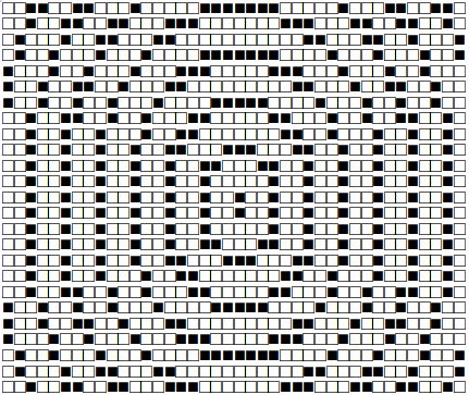
Structured sequence

APPENDIX II.

Algorithms for Minimum and Maximum Information.

public class MinInfo{

	public double minInfo(Collection values){
		if (values == null) {
			return 0;
		}
		if (values.isEmpty()) {
			return 0;
		}
		if (values.size() == 1) {
			return 1;
		}
		return Math.log(values.size() + 1) / Math.log(2);
	}

}

public class MaxInfo{

	public double maxInfo(Collection values){ 
		if (values == null) { 
			return 0; 
		}
		if (values.isEmpty()) 
		{ 
			return 0; 
		} 
		if (values.size() == 1) {
			return 1; 
		} 
		Set atomicSet = new HashSet<>(values); 
		int k = atomicSet.size();
		int n = values.size();
		double v = n * Math.log(k) / Math.log(2);
		if (v > 500) {
			return v;
		} 
		if (k == 1) {
			return Math.log(n + 1) / Math.log(2); 
		}
		return Math.log(
			(Math.pow(k, n + 1) - 1) / (k - 1)) / Math.log(2);
	}

}

APPENDIX III.

Algorithm for the Modified Shannon Information of a Pattern.

public class ModifiedShannonInfo{

	public double modifiedShannonInfo(Collection values) {
		if (values == null || values.isEmpty()) {
	    	return 0;
		}
		if (values.size() == 1) {
			return 1;
		}
		Map<Object, Double> map = new HashMap<>();      
		for (Object x : values) {
			Double frequency = map.get(x);
			if (frequency == null) {
				map.put(x, 1.0);
			} else {
				map.put(x, frequency + 1);
			}
		}
		int n = values.size();
		if (n > 100) {
			return shannonInfo.value(values);
		}
		if (map.size() == 1) {
			return Math.log(n + 1) / Math.log(2);
		}
		for (Object x : map.keySet()) {
			map.put(x, map.get(x) / n);
		}
		double info = 0;
		for (int i = 0; i < n; i++) {
			double p = 1;
			for (Object x : map.keySet()) {
				double f = map.get(x);
				p *= Math.pow(f, -i * f);
			}
			info += p;
		}
		return Math.log(info) / Math.log(2);
	}

}

APPENDIX IV.

Algorithm for the Information of a Pattern Measured by the GZip Compression Algorithm.

public class GZipInfo{

	private final MinInfo minInfo = new MinInfo();
	private final MaxInfo maxInfo = new MaxInfo();

	public double gZipInfo(Collection values) {
		if (input == null || input.size() <= 1) {
		return 0;
		}
	
		byte[] values = ObjectUtils.serialize(input);
	
		double gzipInfo = ArrayUtils.toGZIP(values).length * 8;
	
		double min = minInfo.minInfo(input);
		double max = maxInfo.maxInfo(input);
	
		double minGzipInfo = ArrayUtils.toGZIP(
			new byte[values.length]).length * 8;
		double maxGzipInfo = ArrayUtils.toGZIP(
			generateRandomByteArray(values)).length * 8;
	
		if (originalMax == originalMin) {
			return (newMin + newMax) / 2;
		}
	
		return newMin + ((gzipInfo - minGzipInfo) 
			/ (maxGzipInfo - minGzipInfo)) * (max - min);
	}

}

The Information Content and Entropy of Finite Patterns from a Combinatorial Perspective

1 Introduction

2 Information Content of a Constant Pattern

3 Information Content of a Uniformly Distributed Random Pattern

4 Information Content of Patterns Generated by an Ergodic Markov Process

5 Information Content of General Patterns

5.1 General Properties of Information

5.2 Calculating Information Based on Kolmogorov Complexity

5.3 Calculating Information Based on a Compression Algorithm

6 Entropy of Finite Patterns

7 Summary

References

Leave a Reply Cancel reply

Prespa

Need Help?

Learn More

Get in Touch